Executive Summary
Youtube Video (Open directly)
Introduction:
Picture this: You're standing at a busy coffee shop, watching customers arrive seemingly at random. Some mornings, there's barely a soul; other days, the line snakes out the door. Is there a pattern hidden in this chaos? And more importantly, how can you prove it? Welcome to the fascinating world of probability theory and hypothesis testing—the mathematical framework that helps us not only understand uncertainty but also validate our understanding with statistical rigor.

Part I: The Foundation - Making Sense of Randomness
Understanding Probability Theory
At its core, probability theory is humanity's attempt to quantify the unpredictable. It's the mathematical language we use to describe chance, offering tools to measure likelihood and make informed decisions when faced with uncertainty.
Think of rolling a die. We intuitively know each face has an equal chance of appearing—a 1 in 6 probability, or about 16.67%. But this simple example illustrates profound principles:
- Sample Space (S): All possible outcomes {1, 2, 3, 4, 5, 6}
- Event (E): Any subset, like "rolling an even number" {2, 4, 6}
- Probability P(E): The likelihood of an event occurring (3/6 = 0.5 for even numbers)
These concepts scale from dice games to complex systems. When Amazon predicts what products you'll buy, when your doctor assesses your health risks, or when Netflix recommends your next binge-watch, they're all using these same fundamental principles—just with more sophisticated mathematics.
The Three Axioms That Rule Probability
Everything in probability theory rests on three bedrock principles, formulated by Russian mathematician Andrey Kolmogorov:
- Non-negativity: For any event A, P(A) ≥ 0. Probabilities cannot be negative.
- Normalization: P(S) = 1. The probability of the entire sample space equals one.
- Additivity: For mutually exclusive events A and B, P(A ∪ B) = P(A) + P(B).
These axioms might seem obvious, but they're powerful enough to derive all of probability theory—from simple coin flips to complex financial derivatives.
The Building Blocks: Probability Distributions
Just as architects need blueprints, data scientists and analysts need probability distributions—mathematical descriptions of how likely different outcomes are. These come in two main flavors:
Discrete Distributions: When You Can Count It
Real-world example: A call center receives customer complaints. The manager notices:
- Monday: 23 calls
- Tuesday: 19 calls
- Wednesday: 25 calls
- Thursday: 18 calls
- Friday: 22 calls
The number of calls is discrete—you can't receive 22.7 calls. This data likely follows a Poisson distribution with an average (λ) of about 21.4 calls per day.
Key insight: For a true Poisson distribution, the variance equals the mean exactly. In practice, if your sample variance ≈ sample mean (both around 21-22), this suggests a Poisson pattern. Real-world data often only approximates this theoretical property due to sampling variation.
Continuous Distributions: When Precision Matters
Real-world example: A pharmaceutical company manufactures pills with a target weight of 500mg. Measuring 1,000 pills, they find:
- Average weight: 499.8mg
- Standard deviation: 2.1mg
- Distribution shape: Symmetric bell curve
This follows a normal distribution. Using the 68-95-99.7 rule:
- 68% of pills weigh between 497.7mg and 501.9mg
- 95% weigh between 495.6mg and 504.0mg
- 99.7% weigh between 493.5mg and 506.1mg
This knowledge helps set quality control limits and minimize waste.
Common Distributions in Action
The Binomial Distribution: Success and Failure
Example: A tech startup's sales team makes cold calls with a 15% success rate. If they make 20 calls, what's the probability of getting exactly 3 sales?
Using the binomial distribution:
- n = 20 (trials)
- p = 0.15 (success probability)
- P(X = 3) ≈ 0.243 or 24.3%
Important clarification about binomial variance:
- Variance = np(1-p) = 20 × 0.15 × 0.85 = 2.55
- Mean = np = 3
The relationship between variance and mean in binomial distributions depends on p:
- When p < 0.5: variance > mean
- When p = 0.5: variance = mean/2
- When p > 0.5: variance < mean
This relationship serves as a diagnostic feature for identifying binomial distributions.
Business application: This helps set realistic sales targets. Getting 6 or more sales (double the expected 3) has only a 4% chance—important for compensation planning.
The Poisson Distribution: Counting Random Events
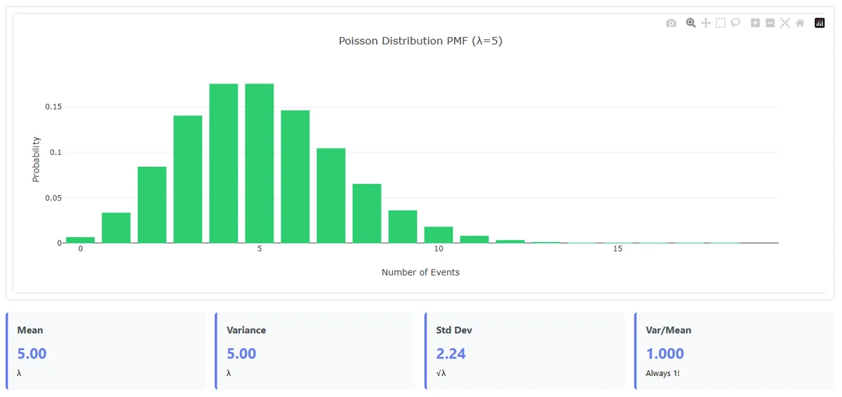
Example: A city's emergency dispatch center tracks ambulance calls:
Midnight to 6 AM: Average 2.5 calls per hour
- Probability of 0 calls in an hour: e^(-2.5) ≈ 8.2%
- Probability of exactly 3 calls: (2.5³ × e^(-2.5))/3! ≈ 21.4%
- Probability of 6+ calls (crisis level): ≈ 4.2%
Key insight about Poisson processes: The Poisson distribution assumes events occur independently with constant rate. What might appear as "clustering"—like getting 5 calls in one hour followed by 0 in the next—is actually expected random variation, not true dependence between events. The process is memoryless: past events don't influence future occurrences.
Tech application: AWS uses Poisson models for auto-scaling. If server requests average 1,000/minute but can spike to 1,500/minute (99th percentile), they provision accordingly.
The Geometric Distribution: Waiting for Success
Example: A quality inspector checks products until finding a defect. If each product has a 2% defect rate:
Expected value vs. probability—an important distinction:
- Expected (mean) products before first defect: 1/0.02 = 50
- Probability of finding defect within first 10 items: 1 - (0.98)^10 ≈ 18.3%
- Probability of checking 100+ items before finding defect: (0.98)^100 ≈ 13.3%
Memoryless property clarified: If you've already checked 50 items without finding a defect:
- The expected number of additional items to check is still 50
- The probability of finding at least one defect in the next 50 items is 1 - (0.98)^50 ≈ 63.6%
This illustrates the difference between expectation (average outcome) and probability (likelihood of specific events).
The Normal Distribution: The Universal Pattern

Deep dive example: A university analyzes 10,000 student exam scores:
- Mean: 72%
- Standard deviation: 12%
This creates grade boundaries:
- A (85%+): Top 14% of students
- B (73-84%): Next 34%
- C (61-72%): Middle 34%
- D (49-60%): Next 14%
- F (<49%): Bottom 2.5%
Why normal appears everywhere: The Central Limit Theorem states that when many independent factors combine additively, the result tends toward normality. A student's exam score combines:
- Natural ability
- Study time
- Sleep quality
- Test anxiety
- Question difficulty
- Random guessing
Each factor contributes to the final score. Combined, they create the bell curve.
Part II: The Detective Work - Hypothesis Testing
When Data Meets Theory: The Need for Statistical Testing
Now comes the crucial question: How do we know if our data actually follows the distribution we think it does? This is where hypothesis testing becomes your statistical detective toolkit.
Imagine you're that quality control manager at the pharmaceutical company. Your pill-making machine is supposed to produce tablets weighing exactly 500mg. You've collected data from 1,000 pills and found they follow a nice bell curve with a mean of 499.8mg. But is this close enough to claim your process is working correctly, or is something systematically wrong?
The Framework: Setting Up Your Investigation
Hypothesis testing follows a courtroom model where we assume innocence (the null hypothesis) until proven guilty beyond reasonable doubt:
Null Hypothesis (H₀): Your default assumption
- "The machine produces 500mg pills"
- "Customer arrivals follow a Poisson distribution"
- "Test scores are normally distributed"
Alternative Hypothesis (H₁): What you conclude if evidence contradicts H₀
- "The machine is miscalibrated"
- "Arrivals don't follow Poisson patterns"
- "Scores aren't normally distributed"
Critical insight: In goodness-of-fit testing, we're always conducting right-tailed tests. The test statistic measures "badness of fit"—larger values indicate worse agreement between data and theory.
The Decision Process: From Evidence to Verdict
The statistical decision-making process follows two equivalent approaches:
| Method | What it gives | Decision Rule |
|---|---|---|
| Critical value | Threshold for test statistic | Reject H₀ if statistic > threshold |
| p-value | Probability of observing data if H₀ true | Reject H₀ if p < α |
Significance Level (α): Your tolerance for Type I error (false positive)
- α = 0.05: Willing to wrongly reject a true H₀ 5% of the time
- α = 0.01: More conservative, only 1% false positive rate
- α = 0.10: More liberal, accepting 10% error rate
Remember: Failing to reject ≠ Proving H₀ true (just like "not guilty" ≠ "innocent")
Goodness-of-Fit Testing: Three Complementary Approaches
1. Chi-Square Test: The Frequency Comparator
How it works: Divides data into bins and compares observed vs. expected counts
Formula: χ² = Σ[(Observed - Expected)²/Expected]
Real-world example: A casino suspects a roulette wheel is biased. In 3,800 spins:
- Red appears 2,050 times (expected: 1,800 for fair wheel)
- Black appears 1,750 times (expected: 2,000)
Calculation:
- χ² = (2050-1800)²/1800 + (1750-2000)²/2000 = 65.95
- Degrees of freedom = categories - 1 = 2 - 1 = 1
- Critical value at 99% confidence with df=1: 6.635
- Conclusion: Wheel is definitely biased (χ² = 65.95 >> 6.635)
When to use:
- Categorical or binned continuous data
- Large sample sizes (n > 50)
- When you can tolerate subjective binning choices
2. Kolmogorov-Smirnov Test: The Distribution Comparator
How it works: Finds the maximum distance between observed and theoretical cumulative distribution functions
Formula: D = max|F_observed(x) - F_theoretical(x)|
Real-world example: An e-commerce site tracks time between orders, hypothesizing exponential distribution with mean 5 minutes. The K-S test compares cumulative distributions:
- Maximum deviation D = 0.089
- Critical value (95%, n=200): 0.096
- Conclusion: Data consistent with exponential (D < critical)
When to use:
- Continuous distributions
- When you want to avoid binning decisions
- For distribution-free comparisons
3. Anderson-Darling Test: The Tail-Sensitive Detector
How it works: Weighted comparison giving extra attention to distribution tails
Formula: A² = -n - Σ[(2i-1)/n][ln(F₀(X₍ᵢ₎)) + ln(1-F₀(X₍ₙ₊₁₋ᵢ₎))]
Real-world example: A risk manager tests whether portfolio returns follow normal distribution. For 250 daily returns:
- A² statistic: 1.24
- Critical value (95%): 0.752
- Conclusion: Reject normality—the distribution has "fat tails"
This finding changes everything: standard risk models underestimate extreme events. The manager must use alternative approaches like Value at Risk with empirical distributions.
When to use:
- Testing normality or other specific distributions
- When tail behavior matters most
- For detecting subtle departures from hypothesized distributions
From Theory to Practice: Integrated Applications
Healthcare: Drug Trial Design
A pharmaceutical company tests a new diabetes medication:
- Control group: 28% show improvement
- Treatment group: Target 40% improvement (clinically significant)
Using binomial distribution and power analysis:
- To detect this difference with 90% power
- At 95% confidence level
- Need approximately 280 patients per group
Then, using chi-square test to validate results:
- If observed improvement is 38% in treatment vs. 29% in control
- χ² = 5.84, df = 1, p-value = 0.016
- Conclusion: Statistically significant improvement
This integrated approach saves millions in trial costs while ensuring reliable results.
E-commerce: Inventory Management
An online retailer sells specialty coffee. Daily demand analysis:
- Identify distribution: Mean = 45, Variance = 43 → Poisson likely
- Validate with K-S test: D = 0.052 < 0.089 (critical) → Accept Poisson
- Apply for inventory:
- For 99% service level: Stock = 45 + 2.33 × √45 ≈ 61 units
- Safety stock = 16 units
This balances customer satisfaction with inventory costs.
Technology: System Reliability
A cloud service uses redundant servers. Analysis process:
- Model failures: Each server uptime follows exponential distribution
- Test with Anderson-Darling: Focus on tail events (extended outages)
- Calculate system reliability:
- Single server downtime: 1%
- Three redundant servers: 0.01³ = 0.000001 or 0.0001%
- System uptime: 99.9999% (six nines)
This calculation justifies the infrastructure investment.
Advanced Considerations: When Theory Meets Reality
The Black Swan Problem
Financial markets don't follow perfect normal distributions. The 2008 crisis occurred in what models considered a "25-sigma event"—theoretically impossible under normal assumptions. Real markets have:
- Fat tails (extreme events more common)
- Volatility clustering (calm breeds calm, chaos breeds chaos)
- Asymmetry (crashes faster than rallies)
Solution: Use Anderson-Darling test to detect fat tails, then apply alternative distributions (Student's t, stable distributions) for risk modeling.
The Multiple Testing Problem
When conducting multiple hypothesis tests, the probability of false positives accumulates:
- Testing 20 independent hypotheses at α = 0.05
- Expected false positives: 20 × 0.05 = 1
- Probability of at least one false positive: 1 - 0.95²⁰ = 64%
Solutions:
- Bonferroni correction: Use α/n for each test
- False Discovery Rate (FDR) control
- Sequential testing procedures
Limitations of Statistical Significance
Large sample paradox: With thousands of observations, even trivial differences become "statistically significant"
- n = 10,000: A correlation of 0.02 might be "significant"
- But is it practically meaningful?
Best practice: Report effect sizes alongside p-values, consider practical significance, not just statistical significance.
A Complete Analysis Framework
Step 1: Exploratory Data Analysis
- Plot histogram
- Calculate mean, variance, skewness, kurtosis
- Look for mathematical signatures
- Create Q-Q plots
Step 2: Hypothesize Distribution
- Mean = Variance → Consider Poisson
- Variance relationship with mean → Check binomial (consider p value)
- Bell-shaped and symmetric → Consider Normal
- Right-skewed, starts at 1 → Consider Geometric
Step 3: Estimate Parameters
- Method of moments (quick and simple)
- Maximum likelihood (optimal properties)
- Robust estimation (handles outliers)
Step 4: Test Goodness-of-Fit
- Choose test based on:
- Data type (discrete vs. continuous)
- Sample size
- Importance of tail accuracy
- Calculate test statistics
- Compare with critical values or compute p-values
- Make decision with stated confidence
Step 5: Apply and Monitor
- Use validated distribution for predictions
- Set up control charts
- Monitor for distribution drift
- Revalidate periodically
Practical Tools for Implementation
For those ready to apply these concepts:
Python libraries:
scipy.stats: Distribution fitting and testingstatsmodels: Advanced statistical modelingnumpy/pandas: Data manipulation
Example code structure:
# Fit distribution
params = scipy.stats.norm.fit(data)

# Test goodness-of-fit
statistic, p_value = scipy.stats.kstest(data, 'norm', params)

# Decision
if p_value < 0.05:
    print("Reject normality assumption")
The Power of Integration: Prediction Meets Validation
Understanding both probability distributions and hypothesis testing transforms you from a passive data observer to an active statistical detective. You can:
Predict with Confidence
Once you've validated that customer arrivals follow Poisson(λ=45), you can:
- Predict tomorrow's traffic: P(X > 60) ≈ 2.3%
- Plan staffing: 54 staff handles 95% of scenarios
- Set SLAs: "99% of hours have < 63 customers"
Optimize Operations
Knowing your manufacturing process follows Normal(100, 2):
- Set control limits: 94-106 captures 99.7%
- Minimize waste: Adjust when mean drifts
- Predict yields: 95% meet ±4 unit tolerance
Manage Risk Intelligently
After testing reveals fat-tailed returns:
- Abandon normal-based VaR
- Use empirical percentiles
- Increase capital buffers
- Implement dynamic hedging
Conclusion: Embracing Uncertainty with Precision
We've journeyed from probability's foundational axioms through practical distribution identification, rigorous hypothesis testing, and real-world applications. This integrated framework reveals that uncertainty isn't something to fear—it's something to measure, test, validate, and ultimately harness.
The next time you encounter data, you're equipped with a complete toolkit:
- Identify patterns using mathematical signatures
- Validate assumptions with appropriate statistical tests
- Make predictions with quantified confidence
- Monitor and adapt as patterns evolve
Final Thoughts: Embracing Uncertainty with Confidence
Whether you're ensuring drug safety, optimizing supply chains, managing investment portfolios, or building reliable systems, these tools provide the mathematical rigor to separate signal from noise, pattern from randomness, and knowledge from assumption.
The beauty lies not in eliminating uncertainty but in embracing it with mathematical precision. In a world awash with data, these skills transform overwhelming complexity into actionable insight, turning the hidden mathematics of everyday uncertainty into your competitive advantage.
Ready for the next frontier? Armed with validated probability distributions, you can venture into Monte Carlo simulations—generating synthetic worlds to explore "what-if" scenarios, optimize decisions, and peer into possible futures. Because once you can describe, test, and validate randomness, the next step is learning to generate and control it.
Youtube Video

Youtube Video
Comments 0
No comments yet. Be the first to comment!
Sign in to leave a comment.