Unlocking Efficiency: An In-Depth Look into Linear Programming

Introduction

Imagine you have a factory that produces various products, each requiring different resources. How would you determine the optimal production plan to maximize profit? This is where linear programming (LP) comes into play. LP is a powerful mathematical technique used to optimize outcomes in a wide range of fields, from economics and engineering to logistics and operations management. By formulating problems into linear equations and inequalities, LP helps in making informed decisions that maximize or minimize specific objectives. Let's explore the fundamentals, applications, and benefits of linear programming, supported by real-world examples.

Understanding Linear Programming

Linear programming is a method to achieve the best outcome (such as maximizing profit or minimizing cost) in a mathematical model where the objective function and the constraints are linear. The core idea is to optimize a linear objective function subject to a set of linear equality and inequality constraints. The solution to an LP problem is typically found at the vertices (corners) of the feasible region defined by the constraints.

To solve an LP problem, one typically uses techniques like the simplex method or interior-point methods. The simplex method, developed by George Dantzig in 1947, is a widely used algorithm for solving LP problems. For example, the simplex method was used by the U.S. Air Force to optimize crew scheduling, leading to significant cost savings and improved efficiency. It works by iteratively improving the solution until the optimal point is reached.

Key Concepts in Linear Programming

Key concepts in linear programming include:

• Objective Function: The mathematical expression that represents the goal of the optimization problem, such as maximizing profit or minimizing cost.
• Constraints: The conditions that must be satisfied for the solution to be feasible. These are usually linear inequalities or equalities.
• Decision Variables: The variables that are adjusted to optimize the objective function within the constraints.
• Feasible Region: The set of all possible solutions that satisfy the constraints.
• Optimal Solution: The best solution found within the feasible region.

Understanding these concepts is crucial for effectively applying LP to real-world problems.

Steps to Solve a Linear Programming Problem

Solving a linear programming problem involves several systematic steps. Let's walk through these steps with an example of a manufacturing problem:

Example: A company produces two products, A and B. Each product requires different amounts of labor and material. The company wants to determine the optimal production levels to maximize profit. The costs and revenues are as follows:

• Product A sells for $50 per unit and requires 2 hours of labor and 4 units of material.
• Product B sells for $40 per unit and requires 3 hours of labor and 2 units of material.
• The company has 120 labor hours and 100 units of material available per week.

From these details, the profit per unit for Product A is $50, and for Product B, it is $40.

Step 1: Identify Decision Variables

Identify the variables that you can control to optimize the objective function. In this example, the decision variables are:

• x1: Number of units of product A produced
• x2: Number of units of product B produced

Step 2: Define the Objective Function

Formulate the objective function, which represents the goal of maximizing profit. For instance:

Maximize: Profit = 50x1 + 40x2

This equation represents the profit from producing x1 units of product A and x2 units of product B.

Step 3: Write All Relevant Constraints

Determine the constraints that must be satisfied for the solution to be feasible. For example:

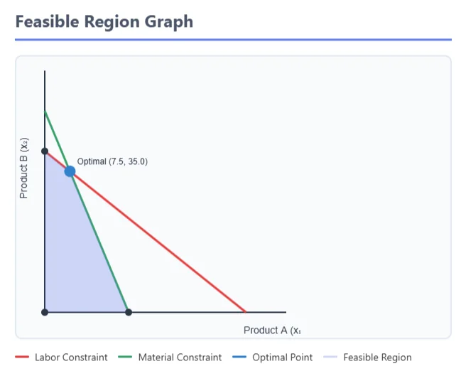
• Labor constraint: 2x1 + 3x2 ≤ 120 (total labor hours available)
• Material constraint: 4x1 + 2x2 ≤ 100 (total material available)
• Non-negativity constraints: x1 ≥ 0, x2 ≥ 0 (production cannot be negative)

Step 4: Convert into Standard or Matrix Form

Convert the objective function and constraints into matrix or standard form for easier computation. This involves setting up the problem in a format suitable for solving algorithms like the simplex method.

Step 5: Solve Using Tools like Excel, R, or Python

Use software tools to solve the problem. For example, Excel's Solver add-in, R's lpSolve package, or Python's PuLP library can be used to find the optimal solution. These tools apply algorithms like the simplex method to find the optimal values of x1 and x2.

Applications of Linear Programming

Linear programming has a vast array of applications across various industries. In logistics, LP can be used to optimize routes for delivery trucks to minimize travel time and fuel costs. For instance, a company like DHL uses LP to optimize its delivery routes, reducing logistics costs by millions of dollars annually. In finance, it helps in portfolio optimization by determining the best mix of assets to maximize returns for a given level of risk. The Black-Scholes model, which uses LP principles, is a well-known example in financial engineering.

In manufacturing, LP aids in production planning by optimizing the use of resources and minimizing costs. For example, companies like Ford Motors use LP to determine the optimal production levels for different car models to meet market demand while minimizing costs. LP is also crucial in healthcare, where it can be used to allocate resources efficiently, such as determining the optimal number of medical staff needed in a hospital to meet patient demands. For example, hospitals in the UK used LP to optimize staffing levels during the COVID-19 pandemic, ensuring that patient care was not compromised. Additionally, in agriculture, LP can help farmers decide the best crop to plant based on available land, labor, and market prices. In India, farmers have used LP to optimize crop planning, leading to increased yields and better profitability.

Furthermore, LP is extensively used in telecommunication for managing network resources. Companies like AT&T use LP to optimize network traffic and reduce congestion, ensuring a better user experience. In energy management, LP helps in scheduling power generation and distribution to meet demand efficiently. For example, power grids use LP to balance supply and demand, ensuring stable and reliable energy distribution. In environmental management, LP can be used to optimize waste disposal and recycling processes to minimize environmental impact.

Benefits of Linear Programming

One of the primary benefits of LP is its ability to provide an optimal solution to complex problems. By systematically evaluating all possible solutions, LP ensures that the best outcome is achieved. This makes it a reliable tool for decision-making in environments where resources are limited and outcomes are critical. Another advantage is its flexibility; LP can be adapted to various types of problems by adjusting the objective function and constraints. For example, a manufacturing company can switch from minimizing costs to maximizing production efficiency by simply changing the objective function.

Moreover, LP solutions are often easy to interpret. The results provide clear guidance on how to allocate resources and make decisions, which is particularly useful in fields where transparency and accountability are important. LP also allows for sensitivity analysis, which helps in understanding how changes in constraints or objectives affect the optimal solution. For instance, in supply chain management, LP helps companies understand how changes in demand or supply affect their logistical plans.

Additionally, LP can handle multiple objectives simultaneously through multi-objective optimization. This allows decision-makers to balance different goals, such as maximizing profit while minimizing environmental impact. For example, in sustainable development, LP can help in creating plans that optimize economic benefits without compromising environmental sustainability.

Challenges and Limitations

Despite its strengths, linear programming has some limitations. One major challenge is that it assumes linearity, which may not always be realistic. Real-world problems often involve non-linear relationships, making LP less accurate in such cases. For example, the cost of production may increase non-linearly with the quantity produced. Additionally, LP can be computationally intensive for very large problems, requiring significant computational resources. The simplex method, while effective, can be slow for large-scale problems.

Another limitation is that LP solutions are often sensitive to the accuracy of input data. Small errors or uncertainties in the data can lead to significantly different optimal solutions. Therefore, careful data collection and validation are essential for reliable LP applications. For example, in financial modeling, small inaccuracies in forecasting future market conditions can lead to suboptimal investment decisions.

Furthermore, LP models can become complex and difficult to manage as the number of variables and constraints increases. This complexity can make it challenging to implement and interpret the results accurately. For instance, in large-scale logistics operations, the number of variables and constraints can be enormous, making the model cumbersome to handle.

Conclusion

Linear programming is a versatile and powerful tool for optimization, with applications across numerous fields. Its ability to provide optimal solutions and its flexibility make it invaluable for decision-making in complex environments. However, it is essential to be aware of its limitations and the need for accurate data. As technology advances, the capabilities of LP continue to expand, making it an even more essential tool for modern optimization challenges. With continuous improvements in algorithms and computational power, LP is poised to play a crucial role in solving increasingly complex optimization problems.

Looking ahead, advancements in machine learning and artificial intelligence are expected to further enhance LP's capabilities. Integrating LP with these technologies can lead to more accurate and efficient solutions, especially in dynamic and uncertain environments. For example, AI can be used to predict future demand and supply patterns, allowing LP to optimize resource allocation more effectively. This synergy between LP and AI holds great promise for addressing some of the most pressing challenges in various industries.

Python Implementation:

from scipy.optimize import linprog
import numpy as np

# Problem parameters
profit_A, profit_B = 50, 40
labor_A, labor_B = 2, 3
material_A, material_B = 4, 2
total_labor, total_material = 120, 100

# Objective function coefficients (negative for maximization)
c = [-profit_A, -profit_B]

# Constraint matrix (Ax <= b)
A = [[labor_A, labor_B],
     [material_A, material_B]]
b = [total_labor, total_material]

# Variable bounds (x >= 0)
x_bounds = [(0, None), (0, None)]

# Solve
result = linprog(c, A_ub=A, b_ub=b, bounds=x_bounds, method='highs')

if result.success:
    x1, x2 = result.x
    max_profit = -result.fun
    print(f"Optimal solution: x1={x1:.2f}, x2={x2:.2f}")
    print(f"Maximum profit: ${max_profit:.2f}")
    
    # Resource utilization
    labor_used = labor_A * x1 + labor_B * x2
    material_used = material_A * x1 + material_B * x2
    print(f"Labor used: {labor_used:.2f}/{total_labor}")
    print(f"Material used: {material_used:.2f}/{total_material}")
else:
    print("No optimal solution found")

# Alternative: Manual corner point method
def corner_point_method():
    corners = [(0, 0)]  # Origin
    
    # Axis intersections
    if total_labor / labor_A >= 0:
        corners.append((total_labor / labor_A, 0))
    if total_labor / labor_B >= 0:
        corners.append((0, total_labor / labor_B))
    if total_material / material_A >= 0:
        corners.append((total_material / material_A, 0))
    if total_material / material_B >= 0:
        corners.append((0, total_material / material_B))
    
    # Constraint intersection
    denom = labor_A * material_B - labor_B * material_A
    if abs(denom) > 1e-10:
        x = (total_labor * material_B - total_material * labor_B) / denom
        y = (total_material * labor_A - total_labor * material_A) / denom
        if x >= 0 and y >= 0:
            corners.append((x, y))
    
    # Filter feasible points
    feasible = []
    for x, y in corners:
        if (x >= 0 and y >= 0 and 
            labor_A * x + labor_B * y <= total_labor + 1e-10 and
            material_A * x + material_B * y <= total_material + 1e-10):
            feasible.append((x, y))
    
    # Find optimal
    best_profit = -1
    best_point = None
    for x, y in feasible:
        profit = profit_A * x + profit_B * y
        if profit > best_profit:
            best_profit = profit
            best_point = (x, y)
    
    return best_point, best_profit

# Compare methods
manual_point, manual_profit = corner_point_method()
print(f"\nManual method: x1={manual_point[0]:.2f}, x2={manual_point[1]:.2f}")
print(f"Manual profit: ${manual_profit:.2f}")